3.4. Datasets

3.4.1. MIT-BIH Arrhythmia Database

We use the MIT-BIH Arrhythmia Database [25] from PhysioNet [16]. The database contains 48 half-hour excerpts of two-channel ambulatory ECG recordings from 47 subjects. The recordings were digitized at 360 samples per second for both channels with 11-bit resolution over a 10mV range. The samples can be read in both digital (integer) form or as physical values (floating point) via the software provided by PhysioNet. We use the integer values in our experiments since our encoder is designed for integer arithmetic. We use the MLII signal (first channel) from each recording in our experiments.

3.4.1.1. Beats

Each beat in the dataset is carefully annotated by a mutual agreement between two cardiologists. There were only a few beats that were very difficult to interpret and were left unclassified by the expert annotators. Different beat annotations found in the dataset and the number of their occurrences across all the 48 records are shown in Table 3.2.

Table 3.2 Beat types

	sym	meaning	counts
0	N	normal beat	75052
1	L	left bundle branch block	8075
2	R	right bundle branch block	7259
3	V	premature ventricular contraction	7130
4	/	paced beat	7028
5	A	atrial premature beat	2546
6	f	fusion of paced and normal beat	982
7	F	fusion of ventricular and normal beat	803
8	j	nodal (junctional) escape beat	229
9	a	aberrated atrial premature beat	150
10	E	ventricular escape beat	106
11	J	nodal (junctional) premature beat	83
12	Q	unclassifiable beat	33
13	e	atrial escape beat	16
14	S	supraventricular premature or ectopic beat (atrial or nodal)	2

3.4.2. Sparsity

In this section, we study the representation of ECG signals in different wavelet bases. The primary goal here is to understand the sparsity pattern of their representations in different bases. If a signal is suitably sparse on an appropriate basis (orthonormal or not), then such a basis can be used effectively for applying an appropriate signal compression method. Towards this, we study the sparsity properties of the wavelet representations of ECG signals in 106 different wavelets from 7 different families. The list of wavelets is provided in Table 3.3.

Table 3.3 List of wavelets

Family	Wavelets
haar	haar
db	db1, db2, db3, db4, db5, db6, db7, db8, db9, db10, db11, db12, db13, db14, db15, db16, db17, db18, db19, db20, db21, db22, db23, db24, db25, db26, db27, db28, db29, db30, db31, db32, db33, db34, db35, db36, db37, db38
sym	sym2, sym3, sym4, sym5, sym6, sym7, sym8, sym9, sym10, sym11, sym12, sym13, sym14, sym15, sym16, sym17, sym18, sym19, sym20
coif	coif1, coif2, coif3, coif4, coif5, coif6, coif7, coif8, coif9, coif10, coif11, coif12, coif13, coif14, coif15, coif16, coif17
bior	bior1.1, bior1.3, bior1.5, bior2.2, bior2.4, bior2.6, bior2.8, bior3.1, bior3.3, bior3.5, bior3.7, bior3.9, bior4.4, bior5.5, bior6.8
rbio	rbio1.1, rbio1.3, rbio1.5, rbio2.2, rbio2.4, rbio2.6, rbio2.8, rbio3.1, rbio3.3, rbio3.5, rbio3.7, rbio3.9, rbio4.4, rbio5.5, rbio6.8
dmey	dmey

3.4.3. Wavelet Comparison Procedure

The following procedure was employed to estimate the sparsity.

For each wavelet and each record

1. Split the record into blocks of \(N=1024\) samples. Let there be \(L\) such blocks.

2. For each \(i\)-th block

   1. Compute the \(N\) point wavelet transform at maximum level.

   2. Sort the wavelet coefficients by magnitude in descending order.

   3. Count the number of largest magnitude coefficients that capture 90% energy of the signal as the number \(k_i\).

3. Put together the sparsity of each block into an array \(K\).

4. Find the maximum, minimum, and mean values of the \(K\) array for the record.

5. Store the \(k_{\max}\), \(k_{\min}\) and \(k_{\text{mean}}\) values against the wavelet name and record number.

A sample of \(k_{\max}\) values for different combinations of wavelets and records is shown in Table 3.4.

Table 3.4 Maximum sparsity for 1024 sized blocks from a few records under a few wavelets

record	rbio3.3	coif7	db14	coif16	haar	coif2	db1	dmey
222	395	226	217	226	311	212	311	219
231	121	96	104	133	128	80	128	100
207	368	210	211	218	341	234	341	218
208	288	165	178	193	248	174	248	172
111	283	164	175	189	245	164	245	169
217	128	95	107	132	131	80	131	96
223	108	84	91	133	111	70	111	88
219	98	86	97	135	90	66	90	87

3.4.4. The Biorthogonal 3.1 Wavelet

Analyzing the data across all records and wavelets, we found that the “bior3.1” wavelet gives the best compressibility performance on average. A sample of the spread of k values from some records with bior3.1 wavelet can be seen in Table 3.5. Among this sample of records, one can see that record 117 appears to be one of the simplest ones as the maximum sparsity level is just 35 while record 200 appears to be one of the complex ones where the sparsity level goes as high as 137. We can also see that in all signals, there are segments that require very few coefficients (20 or less) for almost lossless representation. This is indicative of the fact that when the heart is behaving relatively stably, the ECG pattern is also less complex.

Table 3.5 Sparsity levels of blocks from some records with bior3.1 wavelet

	record	\(k_{\text{mean}}\)	\(k_{\min}\)	\(k_{\max}\)
0	103	36.72	18	53
1	106	34.23	17	68
2	111	37.80	9	98
3	117	22.02	11	35
4	121	18.78	7	44
5	200	39.38	14	137
6	208	36.99	9	113
7	213	41.99	21	62
8	215	52.56	20	114
9	230	37.53	18	63

3.4.5. A Normal Sinus Rhythm

A 1024 sample segment of a normal sinus rhythm in record 102 is depicted in Fig. 3.1. The wavelet coefficients are seen in Fig. 3.2. One can see that about 50 coefficients are needed to capture 99% of the signal energy. Another segment from record 100 in Fig. 3.3 with wavelet coefficients in Fig. 3.4 shows that the sparsity level for normal sinus rhythm can be as low as 21. We haven’t yet established the range of variation in the sparsity level for different types of sinus rhythms under the bior3.1 wavelet.

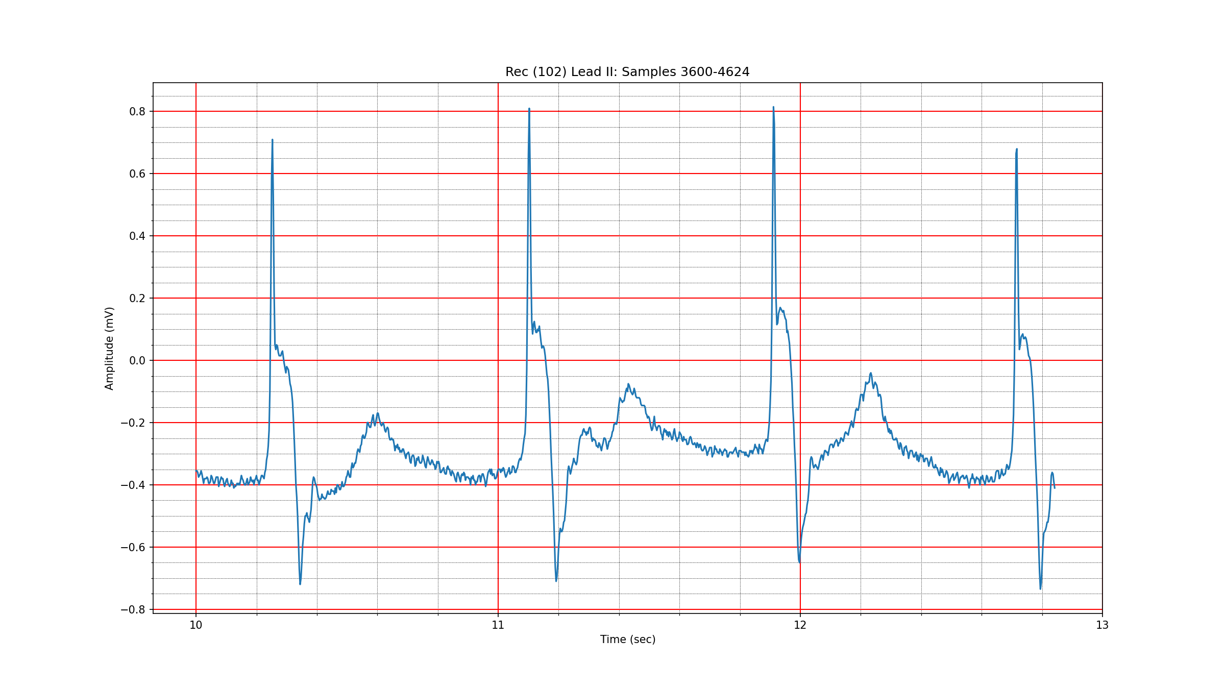
Fig. 3.1 A normal sinus rhythm in record 102

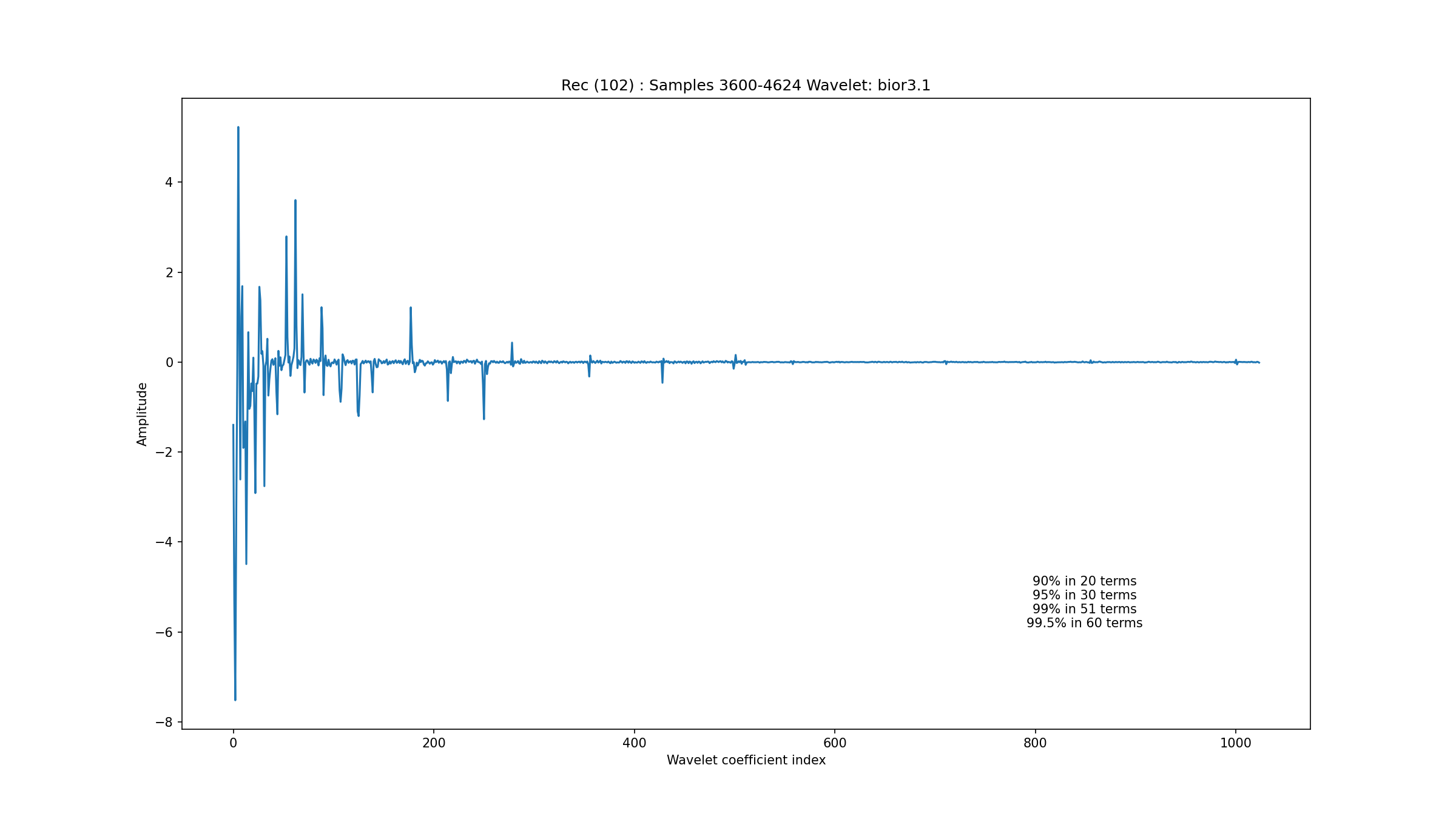
Fig. 3.2 Wavelet coefficients for the normal rhythm in record 102

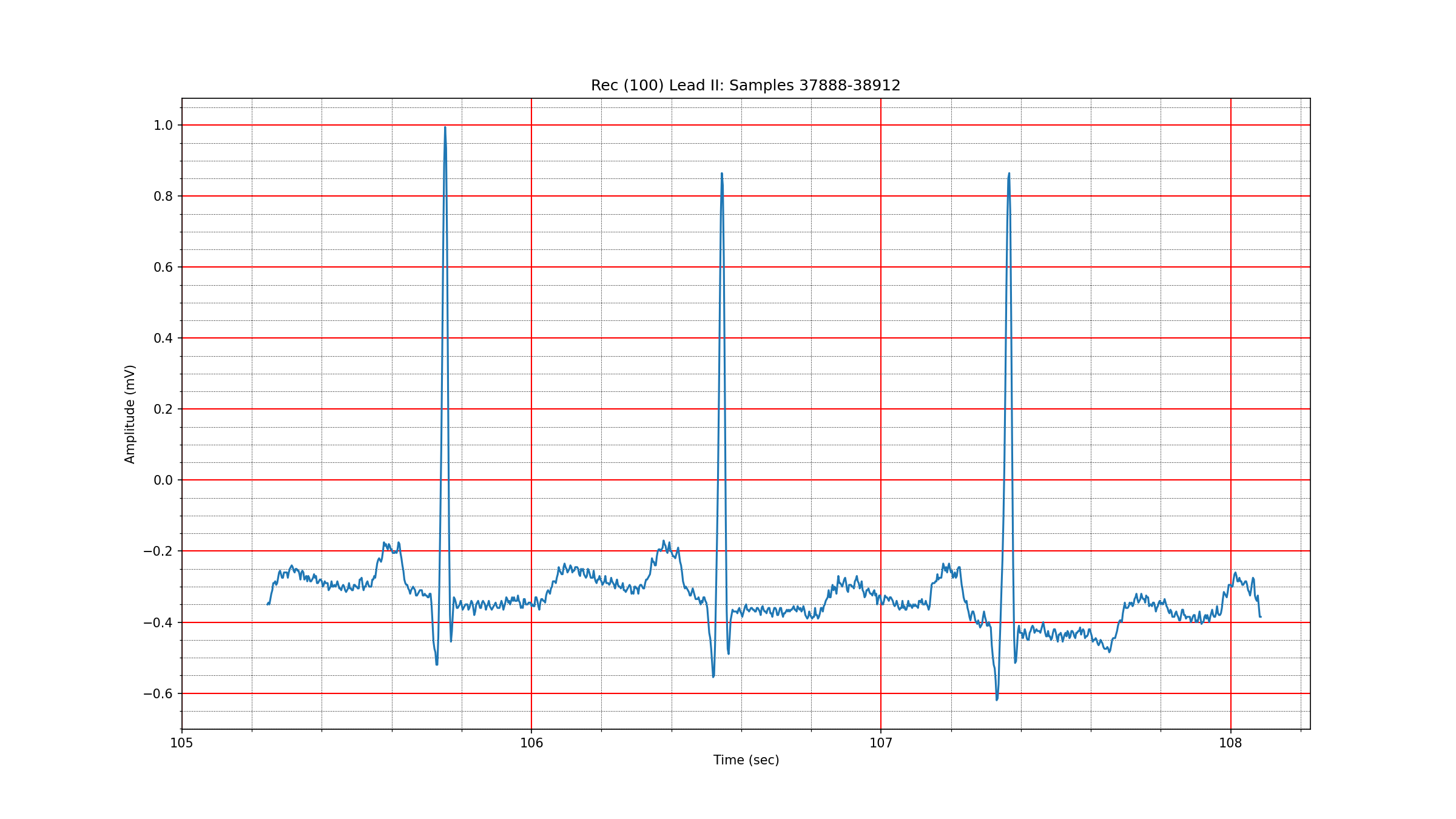
Fig. 3.3 A normal sinus rhythm in record 100

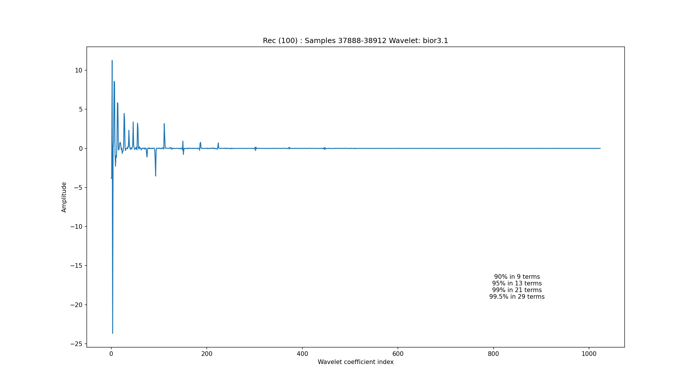
Fig. 3.4 Wavelet coefficients for the normal rhythm in record 100

3.4.6. A Baseline Wander Segment

Fig. 3.5 shows an excerpt of a baseline wander from record 121. It turns out that the wavelet representation for this signal is extremely sparse as seen in Fig. 3.6 with just 7 terms capturing 99% of the energy. One can see that most of the energy in this excerpt is coming from a DC component and a linear trend. This is why this signal has such a highly sparse representation. We noticed that very low sparsity levels tended to correspond to the presence of linear trends in the data.

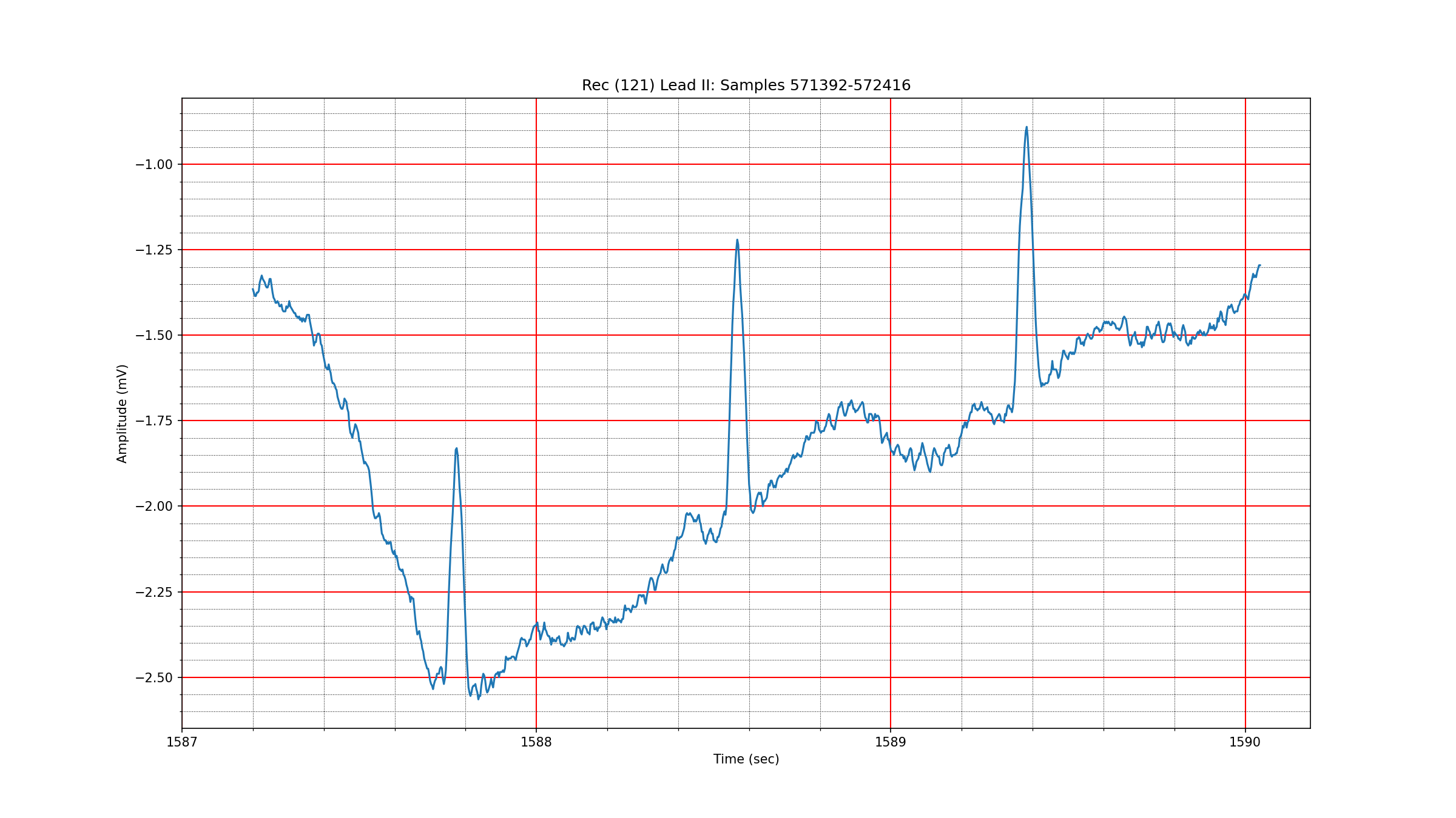
Fig. 3.5 A baseline wander in record 121

Fig. 3.6 Wavelet coefficients for baseline wander in record 121

3.4.7. A Complex ECG Segment

One of the most complex segments of ECG waveforms is found in the record 104 at around \(320\) seconds. This is shown in Fig. 3.7. The corresponding wavelet coefficients using bior3.1 wavelet are shown in Fig. 3.8. As we can see that the wavelet basis is unable to represent this part of the signal sparsely. We need at least \(197\) coefficients to capture 99% energy of the signal. Such signals are very difficult to handle in a compressive sensing framework as they don’t meet the criteria of sparse representation on an appropriate basis. It turns out that this particular segment of ECG is also very hard to interpret. This contains the few beats which remain unclassified to this date in the MIT BIH Arrhythmia dataset.

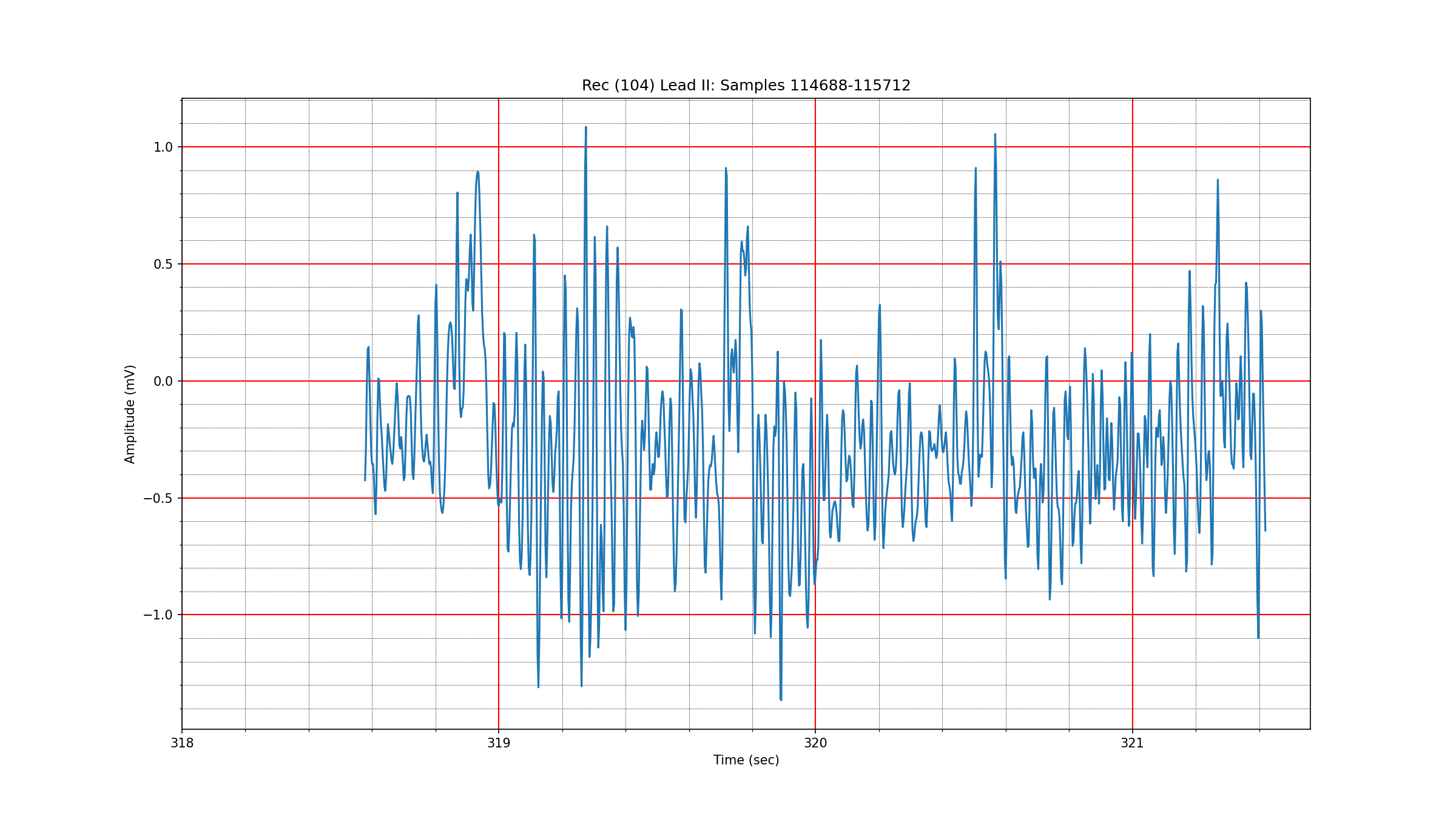
Fig. 3.7 An unclassified ECG segment from record 104

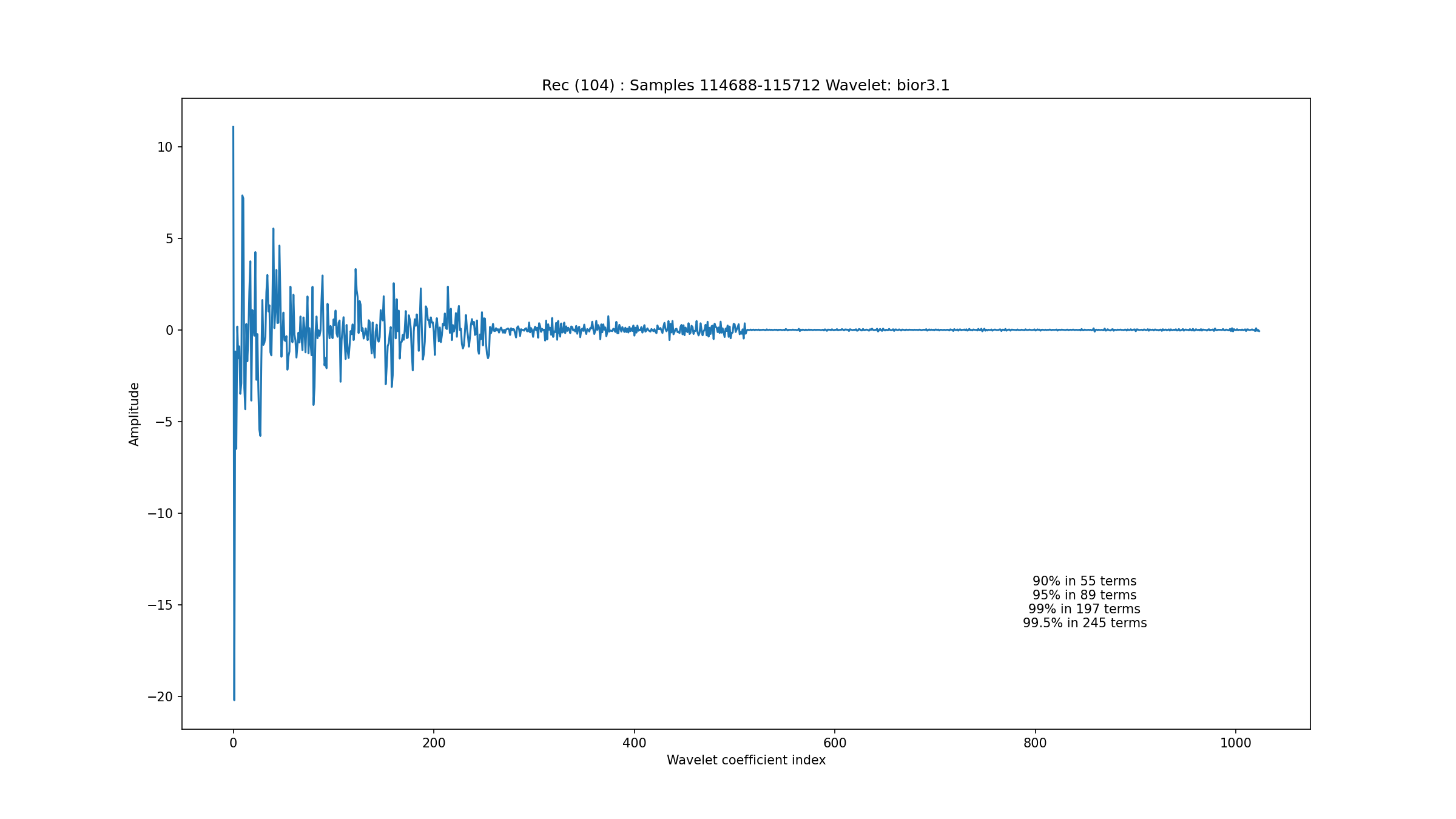
Fig. 3.8 The wavelet coefficients for the unclassified ECG segment from record 104

3.4.8. Sparsity Variation for Different Beat Types

We matched the beat annotations in the dataset with the corresponding 1024 sample blocks and obtained the corresponding sparsity level for 99% energy preservation. We examined the variation of sparsity level in different blocks for individual beat types. This data is provided in Table 3.6. It is interesting to see the significant amount of variation in the sparsity levels for pretty much all beat types. For some beat types, there are too few occurrences to look at the variation in sparsity levels.

Table 3.6 Sparsity level variation for different beat types

	sym	counts	\(k_{\min}\)	\(k_{\max}\)	\(k_{\text{mean}}\)	\(k_{\text{std}}\)
0	N	75052	7	159	36.8	11.4
1	L	8075	9	127	33.3	8.8
2	R	7259	12	134	37.0	11.9
3	V	7130	9	137	33.8	9.0
4	/	7028	15	158	36.5	10.6
5	A	2546	10	130	44.6	13.3
6	f	982	17	197	41.0	17.2
7	F	803	9	97	38.4	7.7
8	j	229	18	152	39.9	17.8
9	a	150	16	54	33.0	6.8
10	E	106	15	47	23.2	5.5
11	J	83	19	56	35.9	10.9
12	Q	33	14	197	88.1	71.2
13	e	16	24	37	31.5	4.2
14	S	2	47	47	47.0	0.0