4.1. Architecture

4.1.1. Problem Statement

We consider the problem of efficient transmission of compressive measurements of ECG signals over the wireless body area networks under the digital compressive sensing paradigm. Let $\mathbf{x}$ be an ECG signal and $\mathbf{y}$ be the corresponding stream of compressive measurements. Our goal is to transform $\mathbf{y}$ into a bitstream $\mathbf{s}$ with as few bits as possible without losing the signal reconstruction quality.

We consider whether a digital quantization of the compressive measurements affects the reconstruction quality. Further, we study the empirical distribution of compressive measurements to explore efficient ways of entropy coding of the quantized measurements.

A primary constraint in our design is that the encoder should avoid any floating point arithmetic so that it can be implemented efficiently in low-power devices.

4.1.2. Block Diagram

Fig. 4.1 presents the high-level block diagram of the proposed encoder.

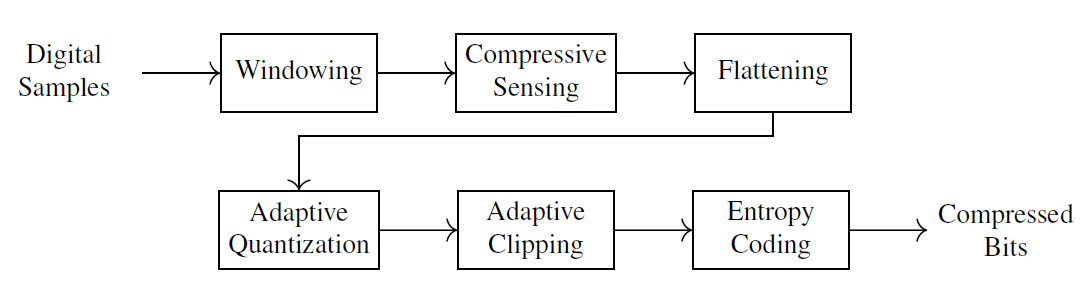
Fig. 4.1 Digital Compressive Sensing Encoder

The ECG signal is split into windows of $n$ samples each. The windows of the ECG signal are further grouped into frames of $w$ windows each. The last frame may have less than $w$ windows. The encoder compresses the ECG signal frame by frame. The encoder converts the ECG signal into a bitstream and the decoder reconstructs the ECG signal from the bitstream.

A window of the signal is the level at which the compressive sensing is done. A frame (a sequence of windows) is the level at which the adaptive quantization is applied and compressed signal statistics are estimated.

The encoding algorithm is further detailed in Algorithm 4.2.

Fig. 4.2 is a high-level block diagram of the proposed decoder.

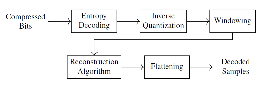
Fig. 4.2 Digital Compressive Sensing Decoder

The decoding algorithm is further detailed in Algorithm 4.3.

4.1.3. Bitstream Format

The encoder first sends the encoder parameters in the form of a stream header (Table 4.1). Then for each frame of the ECG signal, it sends a frame header (Table 4.2) followed by a frame payload consisting of the entropy-coded measurements for the frame.

Algorithm 4.1 (Bitstream format)

1. Send stream header.

2. While there are more ECG data frames:

   1. Send frame header.

   2. Send encoded frame data.

4.1.3.1. Stream Header

The stream header Table 4.1 consists of all the necessary information required to initialize the decoder. In particular, it contains the pseudo-random generator key that can be used to reproduce the sparse binary sensing matrix used in the encoder by the decoder, the number of samples per window ($n$), the number of measurements per window ($m$), the number of ones per column in the sensing matrix ($d$), and the maximum number of windows in each frame of ECG signal ($w$). It contains a flag indicating whether adaptive or fixed quantization will be used. It contains the limits on the normalized root mean square error for the adaptive quantization ($\rho$) and adaptive clipping ($\gamma$) steps. If fixed quantization is used, then it contains the fixed quantization parameter value ($q$). Both $\rho$ and $\gamma$ in the stream header are encoded using a simple decimal format $a{10}^{-b}$ where $a$ and $b$ are encoded as 4-bit integers.

Table 4.1 Stream header

Parameter	Description	Bits
key	PRNG key for $\mathrm{\Phi }$	64
$n$	Window size	12
$m$	Number of measurements per window	12
$d$	Number of ones per column in sensing matrix	6
$w$	Number of windows per frame	8
adaptive	Adaptive or fixed quantization flag	1
if (adaptive )
$\rho$	$\mathrm{N}\mathrm{RMSE}$ limit for adaptive quantization	8
else
$q$	Fixed quantization parameter	4
$\gamma$	$\mathrm{N}\mathrm{RMSE}$ limit for clipping	8

4.1.3.2. Frame Header

The frame header precedes the encoded data for each frame. It captures the encoding parameters that vary from frame to frame.

Table 4.2 Frame header

Parameter	Description	Bits
${\mu }_y$	Mean value	16
${\sigma }_y$	Standard deviation	16
$q$	Frame quantization parameter	3
$r$	Frame range parameter	4
$n_w$	Windows in frame	8
$n_c$	Words of entropy coded data	16

4.1.4. Encoder

Algorithm 4.2 (Encoder algorithm)

1. Send stream header.

2. Build sensing matrix $\mathrm{\Phi }$.

3. For each frame of ECG signal as $\mathbf{x}$

   1. $\mathbf{X}\leftarrow \mathrm{window}(\mathbf{x})$

   2. $n_w\leftarrow$ number of windows in the frame

   3. Compressive sensing: $\mathbf{Y}\leftarrow \mathrm{\Phi }\mathbf{X}$.

   4. $\mathbf{y}\leftarrow \mathrm{flatten}(\mathbf{Y})$.

   5. Adaptive quantization. For $q=q_{max}\dots q_{min}$ (descending)

      1. $\overline{\mathbf{y}}\leftarrow \lfloor \frac{1}{2^q}\mathbf{y}\rfloor$.

      2. $\tilde{\mathbf{y}}\leftarrow 2^q\overline{\mathbf{y}}$

      3. If $\mathrm{N}\mathrm{RMSE}(\mathbf{y},\tilde{\mathbf{y}})\le \rho$ then stop.

   6. Quantized Gaussian model parameters

      1. ${\mu }_y\leftarrow \lceil \text{mean}(\overline{\mathbf{y}})\rceil$.

      2. ${\sigma }_y\leftarrow \lceil (\text{std}(\overline{\mathbf{y}})\rceil$.

   7. Adaptive range adjustment. For $r=2\dots 8$

      1. $y_{min}\leftarrow {\mu }_y-r{\sigma }_y$.

      2. $y_{max}\leftarrow {\mu }_y+r{\sigma }_y$.

      3. $\hat{\mathbf{y}}\leftarrow \mathrm{clip}(\overline{\mathbf{y}},y_{min},y_{max})$.

      4. If $\mathrm{N}\mathrm{RMSE}(\mathbf{y},\hat{\mathbf{y}})\le \gamma$ then break.

   8. $\mathbf{c}\leftarrow \text{ans\_code}(\hat{\mathbf{y}},{\mu }_y,{\sigma }_y,y_{min},y_{max})$.

   9. $n_c\leftarrow$ number of words in $\mathbf{c}$.

   10. Send frame header(${\mu }_y,{\sigma }_y,q,r,n_w,n_c$).

   11. Send frame payload($\mathbf{c}$).

Here we describe the encoding process for each frame. Fig. 4.1 shows a block diagram of the frame encoding process. The input to the encoder is a frame of digital ECG samples at a given sampling rate $f_s$. In the MIT-BIH database, the samples are digitally encoded in 11 bits per sample (unsigned). Let the frame of the ECG signal be denoted by $\mathbf{x}$. The frame is split into non-overlapping windows of $n$ samples each. We shall denote each window of $n$ samples by vectors ${\mathbf{x}}_i$.

4.1.4.1. Windowing

A frame of ECG consists of multiple such windows (up to a maximum of $w$ windows per frame as per the encoder configuration). Let the windows by denoted by ${\mathbf{x}}_1,{\mathbf{x}}_2,\dots$. Let there be $w$ such windows. We can put them together to form the (signed) signal matrix:

$$\mathbf{X}=\left[\begin{array}{cccc}{\mathbf{x}}_1& {\mathbf{x}}_2& \dots & {\mathbf{x}}_w\end{array}\right].$$

PhysioNet provides the baseline values for each channel in their ECG records. Since the digital samples are unsigned, we have subtracted them by the baseline value ($1024$ for 11-bit encoding). 11 bits mean that unsigned values range from $0$ to $2047$. The baseline for zero amplitude is digitally represented as $1024$. After baseline adjustment, the range of values becomes $[-1024,1023]$.

4.1.4.2. Compressive Sensing

Following [22], we construct a sparse binary sensing matrix $\mathrm{\Phi }$ of shape $m\times n$. Each column of $\mathrm{\Phi }$ consists of exactly $d$ ones and $m-d$ zeros, where the position of ones has been randomly selected in each column. An identical algorithm is used to generate the sensing matrix using the stream header parameters in both the encoder and the decoder. The randomization is seeded with the parameter $\mathrm{key}$ sent in the stream header.

The digital compressive sensing operation is represented as

$${\mathbf{y}}_i=\mathrm{\Phi }{\mathbf{x}}_i$$

where ${\mathbf{y}}_i$ is the measurement vector for the $i$-th window. Combining the measurement vectors for each window, the measurement matrix for the entire frame is given by

$$\mathbf{Y}=\mathrm{\Phi }\mathbf{X}.$$

Note that by design, the sensing operation can be implemented using just lookup and integer addition. The ones in each row of $\mathrm{\Phi }$ identify the samples within the window to be picked up and summed. Consequently, $\mathbf{Y}$ consists of only signed integer values.

4.1.4.3. Flattening

Beyond this point, the window structure of the signal is not relevant for quantization and entropy coding purposes in our design. Hence, we flatten it (column by column) into a vector $\mathbf{y}$ of $mw$ measurements.

$$\mathbf{y}=\text{flatten}(\mathbf{Y}).$$

4.1.4.4. Quantization

Next, we perform a simple quantization of measurement values. If fixed quantization has been specified in the stream header, then for each entry $y$ in $\mathbf{y}$, we compute

$$\overline{y}=\lfloor y/2^q\rfloor .$$

For the whole measurement vector, we can write this as

$$\overline{\mathbf{y}}=\lfloor \frac{1}{2^q}\mathbf{y}\rfloor .$$

This can be easily implemented in a computer as a signed right shift by $q$ bits (for integer values). This reduces the range of values in $\mathbf{y}$ by a factor of $2^q$.

If adaptive quantization has been specified, then we vary the quantization parameter $q$ from a value $q_{max}=6$ down to a value $q_{min}=0$. For each value of $q$, we compute $\overline{\mathbf{y}}=\lfloor \frac{1}{2^q}\mathbf{y}\rfloor$. We then compute $\tilde{\mathbf{y}}=2^q\overline{\mathbf{y}}$. We stop if $\mathrm{N}\mathrm{RMSE}(\mathbf{y},\tilde{\mathbf{y}})$ reaches a limit specified by the parameter $\rho$ in the stream header.

4.1.4.5. Entropy Model

Before we explain the clipping step, we shall describe our entropy model. We model the measurements as samples from a quantized Gaussian distribution which can only take integral values. First, we estimate the mean ${\mu }_y$ and standard deviation ${\sigma }_y$ of measurement values in $\overline{\mathbf{y}}$. We shall need to transmit ${\mu }_y$ and ${\sigma }_y$ in the frame header. We round the values of ${\mu }_y$ and ${\sigma }_y$ to the nearest integer so that they can be transmitted efficiently as integers.

Entropy coding works with a finite alphabet. Accordingly, the quantized Gaussian model requires the specification of the minimum and maximum values that our quantized measurements can take. The range of values in $\overline{\mathbf{y}}$ must be clipped to this range.

4.1.4.6. Adaptive Clipping

The clipping function for scalar values is defined as follows:

$$\begin{array}{r}\mathrm{clip}(x,a,b)\triangleq \{\begin{array}{lll}a& & x\le a\\ b& & x\ge b\\ x& & \text{otherwise}.\end{array}\end{array}$$

We clip the values in $\overline{\mathbf{y}}$ to the range $[{\mu }_y-r{\sigma }_y,{\mu }_y+r{\sigma }_y]$ where $r$ is the range parameter estimate from the data. This is denoted as

$$\hat{\mathbf{y}}=\text{clip}(\overline{\mathbf{y}},{\mu }_y-r{\sigma }_y,{\mu }_y+r{\sigma }_y).$$

Similar to adaptive quantization, we vary $r$ from $2$ to $8$ till we have captured sufficient variation in $\overline{\mathbf{y}}$ and $\mathrm{N}\mathrm{RMSE}(\mathbf{y},\hat{\mathbf{y}})\le \gamma$.

4.1.4.7. Entropy Coding

We then model the measurement values in $\hat{\mathbf{y}}$ as a quantized Gaussian distributed random variable with mean ${\mu }_y$, standard deviation ${\sigma }_y$, minimum value ${\mu }_y-r{\sigma }_y$ and maximum value ${\mu }_y+r{\sigma }_y$. We use the ANS entropy coder to encode $\hat{\mathbf{y}}$ into an array $\mathbf{c}$ of 32-bit integers (called words). This becomes the payload of the frame to be sent to the decoder. The total number of compressed bits in the frame payload is the length of the array $n_c$ times 32. Note that we have encoded and transmitted $\hat{\mathbf{y}}$ and not the unclipped $\overline{\mathbf{y}}$. ANS entropy coding is a lossless encoding scheme. Hence, $\hat{\mathbf{y}}$ will be reproduced faithfully in the decoder if there are no bit errors involved in the transmission We assume that an appropriate channel coding mechanism has been used.

4.1.4.8. Integer Arithmetic

The input to digital compressive sensing is a stream of integer-valued ECG samples. The sensing process with the sparse binary sensing matrix can be implemented using integer sums and lookup. It is possible to implement the computation of approximate mean and standard deviation using integer arithmetic. We can use the normalized mean square error-based thresholds for adaptive quantization and clipping steps. ANS entropy coding is fully implemented using integer arithmetic. Thus, the proposed encoder can be fully implemented using integer arithmetic.

4.1.5. Decoder

The decoder initializes itself by reading the stream header and creating the sensing matrix to be used for the decoding of compressive measurements frame by frame.

Algorithm 4.3 (Decoder algorithm)

1. Read stream header.

2. Build sensing matrix $\mathrm{\Phi }$.

3. While there is more data

   1. ${\mu }_y,{\sigma }_y,q,r,n_w,n_c\leftarrow$ read frame header.

   2. $\mathbf{c}\leftarrow$ read frame payload $(n_c)$.

   3. Compute entropy model parameters

      1. $y_{min}\leftarrow {\mu }_y-r{\sigma }_y$.

      2. $y_{max}\leftarrow {\mu }_y+r{\sigma }_y$.

   4. $\hat{\mathbf{y}}\leftarrow \text{ans\_decode}(\mathbf{c},{\mu }_y,{\sigma }_y,y_{min},y_{max})$.

   5. Inverse quantization:

      1. $\tilde{\mathbf{y}}\leftarrow 2^q\hat{\mathbf{y}}$.

      2. $\tilde{\mathbf{Y}}\leftarrow \mathrm{window}(\tilde{\mathbf{y}})$.

      3. $\tilde{\mathbf{X}}\leftarrow \mathrm{reconstruct}(\tilde{\mathbf{Y}})$.

      4. $\tilde{\mathbf{x}}\leftarrow \mathrm{flatten}(\tilde{\mathbf{X}})$.

Here we describe the decoding process for each frame. Fig. 4.2 shows a block diagram for the decoding process. Decoding of a frame starts by reading the frame header which provides the frame encoding parameters: ${\mu }_y,{\sigma }_y,q,r,n_w,n_c$.

4.1.5.1. Entropy Decoding

The frame header is used for building the quantized Gaussian distribution model for the decoding of the entropy-coded measurements from the frame payload. The minimum and maximum values for the model are computed as:

$$y_{min},y_{max}={\mu }_y-r{\sigma }_y,{\mu }_y+r{\sigma }_y.$$

$n_c$ tells us the number of words ($4n_c$ bytes) to be read from the bitstream for the frame payload. The ANS decoder is used to extract the encoded measurement values $\hat{\mathbf{y}}$ from the frame payload.

4.1.5.2. Inverse Quantization

We then perform the inverse quantization as

$$\tilde{\mathbf{y}}=2^q\hat{\mathbf{y}}.$$

Next, we split the measurements into measurement windows of size $m$ corresponding to the signal windows of size $n$.

$$\tilde{\mathbf{Y}}=\mathrm{window}(\tilde{\mathbf{y}}).$$

We are now ready for the reconstruction of the ECG signal for each window.

4.1.5.3. Reconstruction

The architecture is flexible in terms of the choice of the reconstruction algorithm.

$$\tilde{\mathbf{X}}=\mathrm{reconstruct}(\tilde{\mathbf{Y}}).$$

Each column (window) in $\tilde{\mathbf{Y}}$ is decoded independently. In our experiments, we built a BSBL-BO (Block Sparse Bayesian Learning-Bound Optimization) decoder [35, 36, 37]. Our implementation of BSBL is available as part of CR-Sparse library [18]. As Zhang et al. suggest in [35], block sizes are user-defined, they are identical for all blocks, and no pruning of blocks is applied. Our implementation has been done under these assumptions and is built using JAX so that it can be run on GPU hardware easily to speed up decoding. The only configurable parameter for this decoder is the block size which we shall denote by $b$ in the following. Once the samples have been decoded, we flatten (column by column) them to generate the sequence of decoded ECG samples to form the ECG record.

$$\tilde{\mathbf{x}}=\mathrm{flatten}(\tilde{\mathbf{X}}).$$

4.1.5.4. Alternate Reconstruction Algorithms

It is entirely possible to use a deep learning-based reconstruction network like CS-NET [32] in the decoder. We will need to train the network with $\tilde{\mathbf{y}}$ as inputs and $\mathbf{x}$ as expected output. However, we haven’t pursued this direction yet as our focus was to study the quantization and entropy coding steps in this work. One concern with deep learning-based architectures is that the decoder network needs to be trained separately for each encoder configuration and each database. The ability to dynamically change the encoder/decoder configuration parameters is severely restricted in deep learning-based architectures. This limitation doesn’t exist with BSBL algorithms.

4.1.6. Discussion

4.1.6.1. Measurement statistics

Several aspects of our encoder architecture are based on the statistics of the measurements $\mathbf{y}$. We collected the summary statistics including mean $\mu$, standard deviation $\sigma$, range of values in $\mathbf{y}$, skew and kurtosis for the measurement values for each of the ECG records in the MIT-BIH database. These values have been reported for one particular encoder configuration in Table 4.3. In addition, we also compute the range divided by standard deviation $\frac{\text{rng}}{\sigma }$ and the iqr (inter quantile range) divided by standard deviation $\frac{\text{iqr}}{\sigma }$.

Table 4.3 Measurement statistics at $m=256,n=512,d=4$

rec	${\mu }_y$	${\sigma }_y$	iqr	rng	skew	kurtosis	kld	$\frac{\text{rng}}{\sigma }$	$\frac{\text{iqr}}{\sigma }$
100	-490	224	293	2562	-0.46	3.71	0.05	11.41	1.31
101	-455	287	323	9647	-0.39	15.4	0.13	33.61	1.13
102	-393	197	257	2035	-0.55	3.68	0.05	10.33	1.31
103	-370	286	302	8824	-0.78	15.91	0.16	30.86	1.06
104	-360	231	284	4204	-0.61	5.04	0.07	18.16	1.23
105	-360	347	326	13704	-0.38	22.52	0.24	39.52	0.94
106	-285	271	314	4135	-0.09	4.43	0.05	15.28	1.16
107	-372	625	747	9639	-0.46	4.65	0.06	15.43	1.2
108	-366	422	336	12986	-0.16	22.13	0.36	30.75	0.8
109	-368	335	389	7487	0.19	7.33	0.06	22.32	1.16
111	-262	308	306	11998	-0.91	23.07	0.2	38.99	0.99
112	-1316	539	724	7839	-0.64	4.14	0.09	14.55	1.34
113	-248	337	379	6121	-0.05	5.19	0.06	18.18	1.13
114	-249	219	235	8756	1.15	30.41	0.14	39.91	1.07
115	-781	461	559	9715	-0.82	6.74	0.09	21.07	1.21
116	-1498	875	930	35083	-0.29	22.7	0.22	40.1	1.06
117	-1363	560	748	9179	-0.7	4.38	0.1	16.39	1.34
118	-1373	614	809	10935	-0.55	4.37	0.1	17.81	1.32
119	-1378	629	825	8363	-0.57	3.8	0.07	13.3	1.31
121	-1296	635	763	17012	-1.37	13.12	0.16	26.78	1.2
122	-1350	555	747	7870	-0.55	3.73	0.08	14.18	1.35
123	-1274	514	699	6603	-0.57	3.83	0.08	12.84	1.36
124	-1293	679	829	11886	-0.6	5.42	0.1	17.51	1.22
200	-169	262	288	6285	-0.26	7.71	0.08	24.01	1.1
201	-256	189	196	9986	0.72	55.1	0.16	52.71	1.03
202	-271	262	274	11421	-0.98	32.98	0.16	43.58	1.05
203	-271	472	455	13371	-0.14	15.11	0.2	28.35	0.96
205	-489	234	301	3257	-0.57	4.1	0.06	13.94	1.29
207	-274	339	344	11400	-1.19	18.15	0.22	33.62	1.01
208	-265	427	410	12449	0.38	16.51	0.18	29.13	0.96
209	-264	250	292	4731	-0.55	4.89	0.06	18.95	1.17
210	-251	228	249	7909	0.48	17.22	0.09	34.65	1.09
212	-250	297	336	7232	-0.53	7.26	0.09	24.36	1.13
213	-353	523	635	6528	-0.18	4.03	0.04	12.48	1.21
214	-258	315	369	4248	0.16	4.12	0.04	13.47	1.17
215	-243	209	256	3544	-0.27	4.2	0.04	16.98	1.23
217	-264	459	528	11928	-0.3	8.5	0.09	26	1.15
219	-939	688	811	10727	-0.43	4.63	0.07	15.6	1.18
220	-865	378	503	4731	-0.48	3.66	0.06	12.5	1.33
221	-262	228	270	3000	-0.13	4.1	0.04	13.16	1.18
222	-250	212	252	4327	-0.78	5.71	0.08	20.41	1.19
223	-818	419	529	7449	-0.58	4.95	0.07	17.77	1.26
228	-222	357	294	11962	-0.97	23.96	0.35	33.52	0.82
230	-272	285	308	7044	-0.4	8.63	0.1	24.69	1.08
231	-253	229	278	3250	-0.34	4.21	0.04	14.2	1.21
232	-242	192	243	2951	-0.42	3.98	0.04	15.38	1.27
233	-246	427	480	9636	-0.13	6.47	0.08	22.56	1.12
234	-257	345	316	12002	-0.66	19.78	0.25	34.78	0.92

4.1.6.2. Gaussianity

The key idea behind our entropy coding design is to model the measurement values as being sampled from a quantized Gaussian distribution. Towards this, we measured the skew and kurtosis for the measurements for each record as shown in Table 4.3 for the sensing matrix configuration of $m=256,n=512,d=4$. For a Gaussian distributed variable, the skew should be close to $0$ while kurtosis should be close to $3$. While the skew is not very high, Kurtosis does vary widely. Fig. 4.3-Fig. 4.8 show the histograms of measurement values for 6 different records. Although the measurements are not Gaussian distributed, it is not a bad approximation. The quantized Gaussian approximation works well in entropy coding. It is easy to estimate from the data.

The best compression can be achieved by using the empirical probabilities of different values in $\mathbf{y}$ in entropy coding. However, doing so would require us to transmit the empirical probabilities as side information. This may be expensive. We can estimate the improvement in compression overhead by the use of the quantized Gaussian approximation. Let $\mathbb{P}$ denote the empirical probability distribution of data and let $\mathbb{Q}$ denote the corresponding quantized Gaussian distribution. Bamler in [2] show empirically that the overhead of using an approximation distribution $\mathbb{Q}$ in place of $\mathbb{P}$ in ANS entropy coding is close to the KL divergence $\text{KL}(\mathbb{P}||\mathbb{Q})$ which is given by

$$\text{KL}(\mathbb{P}||\mathbb{Q})=\sum _y\mathbb{P}(y){\log }_2\left(\frac{\mathbb{P}(y)}{\mathbb{Q}(y)}\right).$$

We computed the empirical distribution for $\mathbf{y}$ for each record and measured its KL divergence with the corresponding quantized Gaussian distribution. It is tabulated in the kld column in Table 4.3. It varies around $0.11\pm 0.07$ bits across the 48 records. Thus, the overhead of using a quantized Gaussian distribution in place of the empirical probabilities can be estimated to be $4-18\mathrm{\%}$. One can see that the divergence tends to increase as the kurtosis increases. We determined the Pearson correlation coefficient between kurtosis and kld to be $0.67$.

Fig. 4.9 shows an example where the empirical distribution is significantly different from the corresponding quantized Gaussian distribution due to the presence of a large number of $0$ values in $\mathbf{y}$. Note that this is different from the histogram in Fig. 4.8 where the $\mathbf{y}$ values have been binned into 200 bins.

Also, Fig. 4.3-Fig. 4.8 suggest that the empirical distributions vary widely from one record to another in the database. Hence using a single fixed empirical distribution (e.g. the Huffman code-book preloaded into the device in [22]) may lead to lower compression.

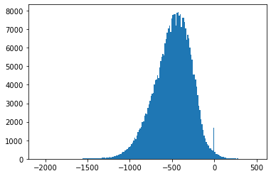
Fig. 4.3 Histograms of measurement values for record 100

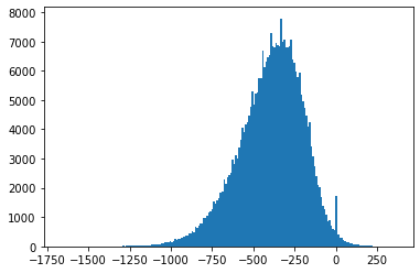
Fig. 4.4 Histograms of measurement values for record 102

Fig. 4.5 Histograms of measurement values for record 115

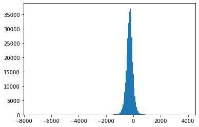
Fig. 4.6 Histograms of measurement values for record 202

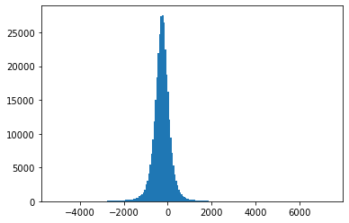
Fig. 4.7 Histograms of measurement values for record 208

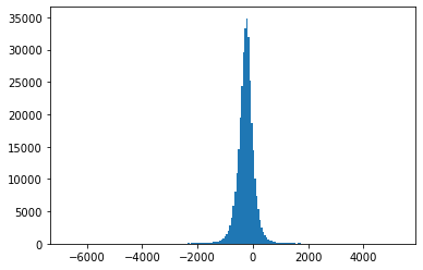
Fig. 4.8 Histograms of measurement values for record 234

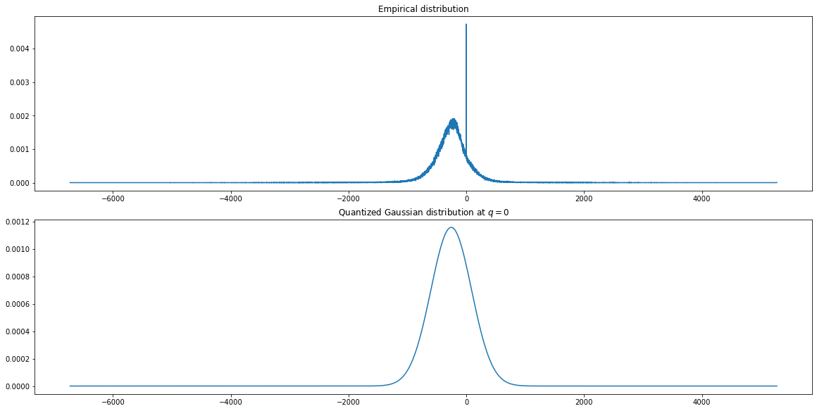
Fig. 4.9 Empirical and quantized Gaussian distributions for measurement values $\mathbf{y}$ in record 234

4.1.6.3. Clipping

An entropy coder can handle a finite set of symbols only. Hence, the range of input values [measurements coded as integers] must be restricted to a finite range. This is the reason one has to choose a distribution with finite support (like quantized Gaussian). From Table 4.3 one can see that while the complete range of measurement values can be up to 40-50x larger than the standard deviation, the iqr is less than $1.5$ times the standard deviation. In other words, the measurement values are fairly concentrated around the mean value. This can be visually seen from the histograms in Fig. 4.3-Fig. 4.8 also.

4.1.6.4. Quantization

Fig. 4.10 demonstrates the impact of the quantization step on the reconstruction quality for record 100 under non-adaptive quantization. $6$ windows of $512$ samples were used in this example. The first panel shows the original (digital) signal. The remaining panels show the reconstruction at different quantization parameters. The reconstruction visual quality is excellent up to $q=5$ (PRD below 7%), good at $q=6$ (PRD at 9%) and clinically unacceptable at $q=7$ (with PRD more than 15%). One can see significant waveform distortions at $q=7$. Also, note how the quality score keeps increasing till $q=4$ and starts decreasing after that with a massive drop at $q=7$.

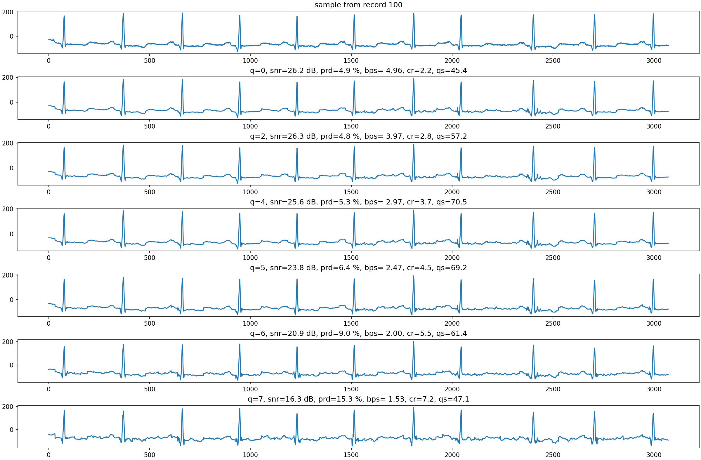
Fig. 4.10 Reconstruction of a small segment of record 100 for different values of $q=0,2,4,5,6,7$ with $m=256,n=512,d=4$ under non-adaptive quantization. Block size for the BSBL-BO decoder is $32$.