Python has excellent support for digital signal processing of ECG signals. In this post, we shall explore some basic capabilities for plotting ECG data and doing some basic signal processing for identifying the R peaks inside the signals.
We shall use NumPy for basic numerical computations
and matplotlib for plotting.
# numerical computations
import numpy as np
# plotting
from matplotlib import pyplot as plt
SciPy includes a sample electrocardiogram signal.
# sample data
from scipy.misc import electrocardiogram
The provided signal is an excerpt (19:35 to 24:35) from the record 208 (lead MLII) provided by the MIT-BIH Arrhythmia Database [1] on PhysioNet [2]. This sample records the heart’s electrical activity at a sampling frequency of 360 Hz.
Let us load the signal
ecg = electrocardiogram()
# Sampling frequency in Hz
fs = 360
Typical ECG strips contain a 10 second snapshot of the signal which provides sufficient information for a quick examination of the heart’s activity. Let us extract a 10 second sample from the beginning.
n = int(fs * 10)
signal = ecg[:n]
# time in sec
ts = np.arange(signal.size) / fs
An ECG strip is organized in major and minor ticks which make it easy for the doctors to quickly estimate the heart rate. Let us write a function to plot an ECG signal accordingly.
def plot_ecg_signal(time, signal):
    fig = plt.figure(figsize=(15, 3));
    ax = plt.axes();
    ax.plot(time, signal);
    # setup major and minor ticks
    min_t = int(np.min(time))
    max_t = round(np.max(time))
    major_ticks = np.arange(min_t, max_t+1)
    ax.set_xticks(major_ticks)
    # Turn on the minor ticks on
    ax.minorticks_on()
    # Make the major grid
    ax.grid(which='major', linestyle='-', color='red', linewidth='1.0')
    # Make the minor grid
    ax.grid(which='minor', linestyle=':', color='black', linewidth='0.5')
    plt.xlabel('Time (sec)');
    plt.ylabel('Amplitude')
    return ax
We can now look at our signal.
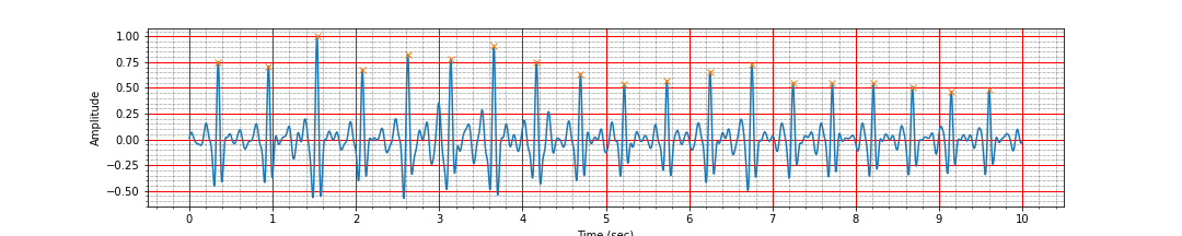
plot_ecg_signal(ts, signal)

Notice how the baseline of the ECG signal is wandering over time. We can see strong R peaks throughout the signal at regular interval. In the following, our goal will be to locate these picks via signal processing and then use the location of R peaks to estimate the heart rate.
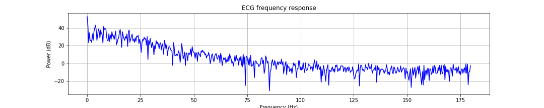
Frequency Spectrum
Most of the frequency components in ECG signals are low frequency. It is worthwhile to examine its frequency spectrum.
from scipy.signal import freqz
w, h = freqz(signal, fs=fs)
fig, ax = plt.subplots(figsize=(15,3))
ax.set_title('ECG frequency response')
ax.plot(w, 20 * np.log10(abs(h)), 'b')
ax.grid()
ax.set_xlabel('Frequency (Hz)')
ax.set_ylabel('Power (dB)')
Finding the R-peaks
SciPy provides a utility function named find_peaks.
The R-peaks in the QRS complexes of an ECG signal are the
most prominent feature. Let us see if we can identify the
peaks directly from the raw ECG signal.
The find_peaks function requires us to provide
some parameters which can be used to distinguish
the prominent peaks from other local maxima. One
is the minimum distance between two peaks. The
other is the height of the peak viz. nearby signal content.
Since there is so much baseline wander happening, the
height is not a reliable factor.
There is a absolute refractory period of 200 ms after an R peak during which no new electrical synapse can be fired in the heart. We can use this to decide the minimum gap (in samples) between two R-peaks.
qrs_refrac_time=200 # ms
n_samp_qrs_refrac = round(qrs_refrac_time * fs / 1000.)
print(n_samp_qrs_refrac)
72
We shall use the minimum distance as well as a threshold of 60% in the range of values of the ECG signal for peak detection in the following function:
def find_r_peaks(time, signal, threshold=0.6, distance=n_samp_qrs_refrac):
    smax = np.max(signal)
    smin = np.min(signal)
    srange = smax - smin
    th = srange * threshold + smin
    r_peaks, _ = find_peaks(signal > th, height=0, distance=distance)
    peak_times = time[r_peaks]
    peak_values = signal[r_peaks]
    return peak_times, peak_values
Using the function to find the peaks:
peak_times, peak_values = find_r_peaks(ts, signal)
We can use the positions of these peaks to estimate a rough average heart rate value:
def compute_hr(peak_times):
    # time difference between peaks
    intervals = np.diff(peak_times)
    n_peaks = peak_times.size
    first_last_interval = peak_times[-1] - peak_times[0]
    mean_heart_rate = (n_peaks - 1) * 60 / first_last_interval
    print(f'Number of peaks {n_peaks}, interval: {first_last_interval:.2f} sec, Average heart rate: {mean_heart_rate:.2f} bpm')
    return mean_heart_rate
Let us estimate the heart rate.
mean_heart_rate = compute_hr(peak_times)
Number of peaks 18, interval: 9.25 sec, Average heart rate: 110.24 bpm
We should check if we identified the peaks correctly by marking the peaks on top of the ECG plot.
ax = plot_ecg_signal(ts, signal)
ax.plot(peak_times, peak_values, 'x');
Ah, a careful inspection shows that we have missed 2 of the peaks between the time 5 and 6 seconds and we have detected a false peak near 8 second. It is time to look for a more robust peak detection algorithm.
Pan Tompkins Algorithm
Pan and Tompkins proposed a famous QRS complex detection algorithm in [3]. The algorithm involves some preprocessing steps on the ECG signal:
- Bandpass filtering
- Differentiation
- Squaring
- Moving average integration
The ECG signal obtained after these steps is far more cleaner
and R peaks are easily identifiable.
Let us see how we can carry out these steps efficiently in
Python.
We shall use signal processing features in SciPy
for these steps:
import scipy as sp
import scipy.signal
Band Pass Filtering
Pan and Tompkins suggest a bandpass filter of 5-15Hz on the input raw ECG signal. Let us design the filter coefficients:
# lower cutoff frequency
f1 = 5
# upper cutoff frequency
f2 = 15
# passband in normalized frequency
Wn = np.array([f1, f2]) * 2 / fs
# butterworth filter
N = 3
b, a = sp.signal.butter(N,Wn, 'bandpass')
Let us now apply the filter and normalize the signal after filtering.
# band pass filter
signal_h = sp.signal.filtfilt(b,a,signal)
# normalize
signal_h = signal_h/ np.max( np.abs(signal_h))
From the perspective of detection of the location of R-peaks, the exact value of the signal doesn’t matter. Only, the form matters. Hence, normalization makes our job easier by limiting the range of ECG signal values.
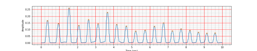
Let us now identify the peaks.
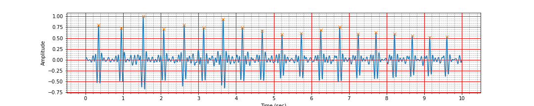
peak_times, peak_values = find_r_peaks(ts, signal_h)
mean_heart_rate = compute_hr(peak_times)
ax = plot_ecg_signal(ts, signal_h)
ax.plot(peak_times, peak_values, 'x');
Number of peaks 19, interval: 9.26 sec, Average heart rate: 116.69 bpm

Voila! After the band pass filtering, we have been able to correctly identify all the peaks. However, we should not be placated by this and carry out the remaining preprocessing tasks also.
Derivative Filter
Pan and Tompkins had originally suggested a derivative
filter with coefficients [1, 2, 0, -2, -1.]. However,
this was suggested for ECG signals sampled at 200Hz.
Since our signal is at 360Hz, we need to revise the
filter coefficients to match this sampling frequency.
The code below does the resampling of the filter coefficients.
# derivative filter
# we need to change the coefficients from 200 Hz sampling rate
# to our sampling rate
# The 200 Hz filter
h = np.array([1, 2, 0, -2, -1.])
# Length of the filter
l = h.size
# new length
l2 = round(fs * l / 200) + 1
# interpolation function
x1 = np.arange(5)
y1 = h*(1/8.0)*fs
f  = sp.interpolate.interp1d(x1,y1)
# new locations
x2 = np.linspace(0, 4, l2)
# new filter coefficients
h = f(x2)
Let us perform derivative filtering.
signal_d = sp.signal.filtfilt(h,1,signal_h)
signal_d = signal_d/np.max(np.abs(signal_d))
Now check the peaks:
peak_times, peak_values = find_r_peaks(ts, signal_d)
mean_heart_rate = compute_hr(peak_times)
ax = plot_ecg_signal(ts, signal_d)
ax.plot(peak_times, peak_values, 'x');
Number of peaks 19, interval: 9.26 sec, Average heart rate: 116.69 bpm
It is all good. No mistakes.
Squaring
Squaring the signal is quite easy:
# squaring the signal
signal_s = signal_d**2
Moving Average Integration
Pan and Tompkins suggested a moving average integration over a period of 150 ms.
Here is the filter for the same:
# Moving average filter length (150 ms)
mvl = round(0.150*fs)
# moving average filter
ma_h = np.ones(mvl) /mvl
Let us perform the moving average integration
# moving average integration
signal_i = sp.signal.convolve(signal_s , ma_h, mode='same')
Let us identify the peaks from this integrated signal
peak_times, peak_values = find_r_peaks(ts, signal_i)
mean_heart_rate = compute_hr(peak_times)
ax = plot_ecg_signal(ts, signal_i)
ax.plot(peak_times, peak_values, 'x');
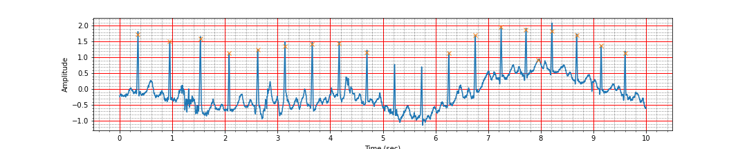
Number of peaks 4, interval: 3.31 sec, Average heart rate: 54.36 bpm
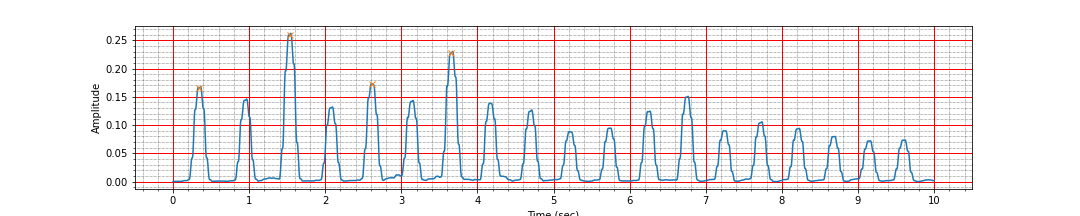
Ah, the signal is clean but we are missing most of the peaks. Turns out that many of the R peaks are much smaller than the largest peak value in this signal. Let us decrease the threshold and check again.
peak_times, peak_values = find_r_peaks(ts, signal_i, threshold=0.2)
mean_heart_rate = compute_hr(peak_times)
ax = plot_ecg_signal(ts, signal_i)
ax.plot(peak_times, peak_values, 'x');
Number of peaks 19, interval: 9.25 sec, Average heart rate: 116.72 bpm
The detection looks good now.
After all this work, we definitely wish if there was a library which would do all this for us so that we don’t have to do all these steps manually. In fact, there are some additional details of the Pan Tompkins algorithm which we have skipped here. It turns out, there is indeed a Python library providing this capability.
WFDB-Python
WFDB-Python is a pure Python library which provides interfaces for accessing the physiological signals in PhysioNet database. It provides functions for reading, writing, processing, and plotting physiologic signal and annotation data. The core I/O functionality is based on the Waveform Database (WFDB) specifications.
It also provides some QRS detection and instantaneous heart rate computation
algorithms. You can install the library using either pip or poetry:
pip install wfdb
poetry add wfdb
Let us import the relevant modules:
import wfdb
from wfdb import processing
GQRS Algorithm
We shall use the GQRS algorithm provided in the library to detect the peaks.
# Use the GQRS algorithm to detect QRS locations in the first channel
qrs_inds = processing.qrs.gqrs_detect(sig=signal, fs=fs)
Once the QRS complexes have been located, we can compute the instantaneous heart rates:
Instantaneous Heart Rate
# Calculate instantaneous heart rate
hrs = processing.hr.compute_hr(sig_len=signal.shape[0], qrs_inds=qrs_inds, fs=fs)
We can now overlay the peak locations and instantaneous heart rates on top of the signal:
figsize=(15, 5)
title="GQRS peak detection"
N = signal.shape[0]
fig, ax_left = plt.subplots(figsize=figsize)
ax_right = ax_left.twinx()
ax_left.plot(ts, signal, color='#3979f0', label='Signal')
ax_left.plot(ts[qrs_inds], signal[qrs_inds], 'x',
             color='#8b0000', label='Peak', markersize=12)
ax_right.plot(ts, hrs, label='Heart rate', color='m', linewidth=2)
ax_left.set_title(title)
ax_left.set_xlabel('Time (sec)')
ax_left.set_ylabel('ECG (mV)', color='#3979f0')
ax_right.set_ylabel('Heart rate (bpm)', color='m')
# Make the y-axis label, ticks and tick labels match the line color.
ax_left.tick_params('y', colors='#3979f0')
ax_right.tick_params('y', colors='m')
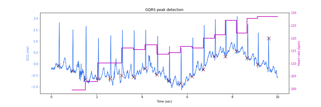
There is a slight problem. The peak locations are somewhat earlier than the actual peaks. This happens due to the different filtering steps in the QRS detection algorithm which lead to some sample delays.
Also note that the instantaneous heart rate calculation skips some cycles as there is not enough data yet to do the computation reliably. The ECG signal amplitude is marked on the left Y axis while the heart rate value is marked on the right Y axis (varying between 100 to 130 beats per minute).
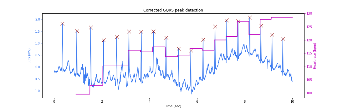
Peak Correction
We can rectify the peak location problem by searching for the correct peaks in the neighborhood of the detected locations. This process is known as the peak correction.
# Correct the peaks shifting them to local maxima
min_bpm = 20
max_bpm = 230
#min_gap = record.fs * 60 / min_bpm
# Use the maximum possible bpm as the search radius
search_radius = int(fs * 60 / max_bpm)
corrected_peak_inds = processing.peaks.correct_peaks(signal,
                                                     peak_inds=qrs_inds,
                                                     search_radius=search_radius,
                                                     smooth_window_size=150)
corrected_peak_inds = sorted(corrected_peak_inds)
We are now ready to plot our detected peaks at correct locations:
figsize=(15,5)
title="Corrected GQRS peak detection"
N = signal.shape[0]
fig, ax_left = plt.subplots(figsize=figsize)
ax_right = ax_left.twinx()
ax_left.plot(ts, signal, color='#3979f0', label='Signal')
ax_left.plot(ts[corrected_peak_inds], signal[corrected_peak_inds], 'x',
             color='#8b0000', label='Peak', markersize=12)
ax_right.plot(ts, hrs, label='Heart rate', color='m', linewidth=2)
ax_left.set_title(title)
ax_left.set_xlabel('Time (sec)')
ax_left.set_ylabel('ECG (mV)', color='#3979f0')
ax_right.set_ylabel('Heart rate (bpm)', color='m')
# Make the y-axis label, ticks and tick labels match the line color.
ax_left.tick_params('y', colors='#3979f0')
ax_right.tick_params('y', colors='m')
References
- Moody GB, Mark RG. The impact of the MIT-BIH Arrhythmia Database. IEEE Eng in Med and Biol 20(3):45-50 (May-June 2001). (PMID: 11446209); DOI:10.13026/C2F305
- Goldberger AL, Amaral LAN, Glass L, Hausdorff JM, Ivanov PCh, Mark RG, Mietus JE, Moody GB, Peng C-K, Stanley HE. PhysioBank, PhysioToolkit, and PhysioNet: Components of a New Research Resource for Complex Physiologic Signals. Circulation 101(23):e215-e220; DOI:10.1161/01.CIR.101.23.e215
- Pan, Jiapu, and Willis J. Tompkins. “A real-time QRS detection algorithm.” IEEE transactions on biomedical engineering 3 (1985): 230-236.